Stationary Processes in Finance
A stationary process is a fundamental concept in time series analysis, and it holds significant importance in finance. In essence, a stationary process is one whose statistical properties, such as mean, variance, and autocorrelation, do not change over time. This doesn’t mean the data values are constant, but rather that their underlying generating mechanism remains consistent across the observation period.
Why is stationarity so crucial in finance? Because many statistical models used for forecasting and analysis rely on the assumption that the data is stationary. If a time series is non-stationary, applying these models directly can lead to spurious results, unreliable predictions, and misleading conclusions. Think of it like trying to predict the trajectory of a ball thrown with a consistent force and angle versus one launched with randomly changing forces and angles. The former is much easier to model accurately.
In financial applications, examples of time series that are often, but not always, considered stationary (or can be transformed to stationarity) include:
- Asset Returns: Daily or monthly returns on stocks, bonds, or other assets are frequently assumed to be stationary. While the price itself is rarely stationary, the *change* in price expressed as a return often exhibits stationary properties.
- Interest Rate Spreads: The difference between two interest rates (e.g., the yield on a corporate bond minus the yield on a government bond) may be stationary, reflecting a relatively stable risk premium.
- Volatility Measures: Certain measures of volatility, such as the VIX index (a measure of market implied volatility), can be analyzed as stationary processes, especially after appropriate transformations.
However, many financial time series are inherently non-stationary. Stock prices, for instance, tend to exhibit trends and random walks. To address this, several techniques are used to achieve stationarity:
- Differencing: Taking the difference between consecutive data points is a common method. First differencing is often enough to render a non-stationary series stationary, especially if the series has a linear trend. Higher order differencing can address more complex trends.
- Detrending: Removing a trend component, typically estimated through regression, can make the residuals stationary.
- Seasonal Adjustment: If the data exhibits seasonality (e.g., quarterly earnings), removing the seasonal component can improve stationarity.
- Transformations: Logarithmic transformations are often used to stabilize the variance of a time series.
Once a time series is rendered stationary, techniques such as ARIMA (Autoregressive Integrated Moving Average) models, Vector Autoregression (VAR) models, and various statistical tests can be applied with greater confidence. These models can then be used for tasks such as forecasting future values, identifying relationships between different time series, and testing hypotheses about market efficiency.
In conclusion, understanding and addressing stationarity is a critical step in any financial time series analysis. Failing to do so can lead to inaccurate models and flawed decision-making. While financial data often presents challenges in terms of stationarity, appropriate techniques can be employed to transform the data, enabling more robust and reliable statistical analysis.
 800×830 process templates finance flowingly from flowingly.io
 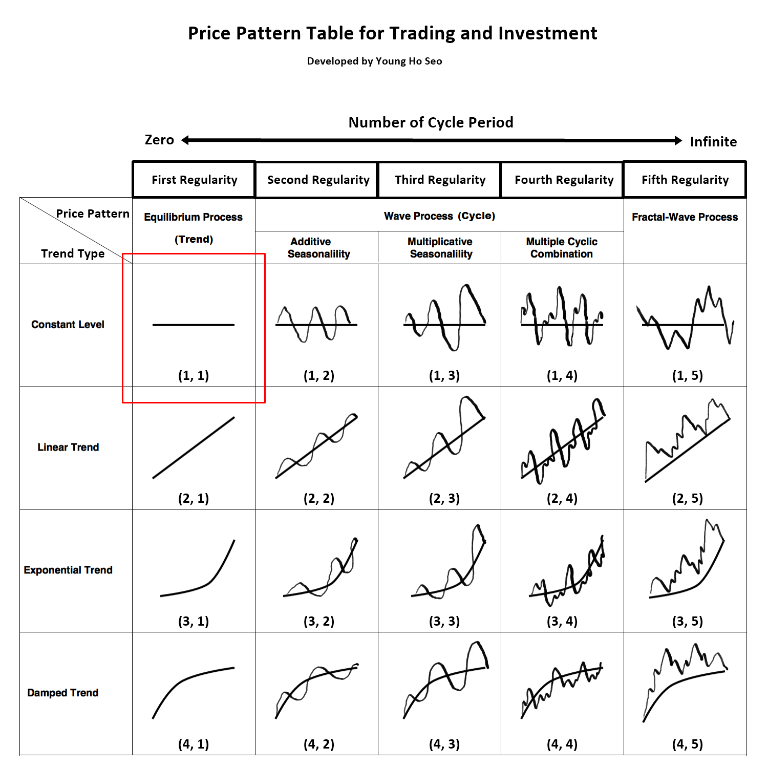 1500×1500 stationary process trend from algotrading-investment.com
 :max_bytes(150000):strip_icc()/AnIntroductiontoStationaryandNon-StationaryProcesses4_4-4faaa0eeb6e84fbc8cebdc1c6b498834.png) 3274×2074 introduction stationary stationary processes from www.investopedia.com
3274×2074 introduction stationary stationary processes from www.investopedia.com  1600×1690 financial process depicted infographic stock vector illustration from www.dreamstime.com
  1302×1335 simple financial process automation software frevvo from www.frevvo.com